Study 1 — Anomaly Detector Sensitivity Analysis
Status: Implemented and executed.
Script: uq/study1_anomaly/run_anomaly_uq.py
Model wrapper: uq/study1_anomaly/anomaly_runner.py
Model under analysis: ai/anomaly_detection.py
For setup instructions and an overview of all studies, see UQ Overview.
Table of Contents
- Background and motivation
- Methodology
- Results
- What the results mean for the HOMEPOT system
- Recommended changes
Background and motivation
The AnomalyDetector class in ai/anomaly_detection.py is responsible for deciding whether a POS device is behaving abnormally. It is called by the AI API layer and its score directly influences what alerts operators see.
The detector reads seven metrics from a device and computes a score between 0.0 (normal) and 1.0 (critical anomaly). Each metric triggers a fixed score addition only when it crosses its threshold:
| Metric | Threshold | Score added if triggered |
|---|---|---|
consecutive_failures | ≥ 3 health check failures | +0.80 |
flapping_count | > 5 state changes/hr | +0.60 |
error_rate | > 5% | +0.50 |
network_latency_ms | > 200ms | +0.40 |
cpu_percent | > 90% | +0.20 |
memory_percent | > 90% | +0.20 |
disk_percent | > 90% | +0.20 |
The score is capped at 1.0. These weights were written by hand and never validated. The key questions are:
- Do the weights reflect the intended relative importance of the metrics?
- Which metrics actually drive the score across the realistic range of device states?
- Is the detector reading its configuration correctly?
Methodology
Polynomial Chaos Expansion (PCE) — a plain-language explanation
Running a model thousands of times at randomly chosen inputs (brute-force Monte Carlo) would answer these questions, but is slow and statistically inefficient. Polynomial Chaos Expansion (PCE) is a smarter alternative: it runs the model at a specific, mathematically optimal set of points, then fits a polynomial approximation to the relationship between inputs and the output. From this polynomial, it can compute statistical summaries analytically — no further model runs needed.
Think of it as fitting a curve to experimental data. Instead of measuring your system at thousands of random conditions, you measure it at a carefully chosen set that allows the best possible curve to be fitted with the fewest points.
With 7 inputs and polynomial order 2, EasyVVUQ's PCE sampler selects 2 187 sample points. Each point is a specific combination of values for all seven metrics. The AnomalyDetector is run once at each point. The PCE fitting and statistical analysis then take milliseconds.
The campaign is orchestrated by run_anomaly_uq.py using the following EasyVVUQ components:
PCESampler— generates the 2 187 input combinationsGenericEncoder— writes each combination toinput.jsonusinganomaly_runner.templateExecuteLocal— runsanomaly_runner.pyonce per sample, which importsAnomalyDetectorfromai/anomaly_detection.pyand writes the result tooutput.jsonJSONDecoder— collects results into the campaign databasePCEAnalysis— fits the polynomial and computes statistics
Sobol Sensitivity Indices — a plain-language explanation
The Sobol first-order sensitivity index for a parameter answers the question: "If I vary only this one parameter — holding everything else constant — what fraction of the total variability in the output is that responsible for?"
An index of 0.499 for consecutive_failures means: ~50% of all the variation in anomaly scores, across all realistic device states, is caused by variation in consecutive_failures alone. An index of 0.000 for cpu_percent means: CPU usage is effectively invisible to the detector in this study — see the saturation paradox discussion in Results for why this can mean either "never fires" or "always fires".
A parameter with an index near zero is effectively invisible to the detector — you could change it significantly and the score would barely move. A parameter with an index near 1.0 almost entirely controls the outcome.
Input distributions
Each metric is given a probability distribution that defines the range of values it can take across the sample space. The choice of distribution and range directly affects which parameters appear sensitive in the Sobol analysis.
Why Uniform? Uniform distributions are used here because there is no prior fleet telemetry to fit against. A Uniform distribution is the maximum-entropy (most agnostic) choice: it assigns equal probability to all values in the range and ensures the Sobol rankings reflect the model's structure, not assumptions about real usage. This is standard practice for an initial sensitivity study.
Uniform may not be appropriate in production. Once real telemetry is available, better-informed distributions should be fitted:
| Parameter | More suitable production distribution | Reason |
|---|---|---|
cpu_percent, memory_percent | Truncated Normal or Beta | Most devices cluster around a typical operating point |
network_latency_ms | Log-Normal | Right-skewed; most devices are fast, with a long tail of slow/degraded links |
error_rate | Beta(α, β) fitted to observed rates | Bounded [0,1]; shape depends on fleet characteristics |
flapping_count, consecutive_failures | Poisson or negative-Binomial | Count data with heavier tails than Uniform |
Switching distributions would shift the absolute Sobol values but the ranking of which parameters matter most is expected to be stable.
How the range affects results — the P(fires) formula.
For a Uniform(a, b) input with a binary threshold check at value \(T\):
Both extremes collapse the Sobol index toward zero:
- Fires rarely (~0%) → the metric almost never changes the score → Sobol ≈ 0
- Fires almost always (~100%) → the metric adds a near-constant offset to every score → variance ≈ 0 → Sobol ≈ 0
The ideal is a P(fires) somewhere in the middle. The ranges below were chosen with this in mind:
| Parameter | Distribution | Range | Threshold | P(fires) | Rationale |
|---|---|---|---|---|---|
cpu_percent | Uniform | 5% – 100% | 90% | ~11% | Wide range so healthy devices (5–80%) dominate; fires only in the tail |
memory_percent | Uniform | 10% – 100% | 90% | ~11% | Same rationale as CPU |
disk_percent | Uniform | 10% – 100% | 90% | ~11% | Same rationale as CPU |
error_rate | Uniform | 0 – 50% | 5% | ~90% | Fires almost always — saturation paradox (see Results) |
network_latency_ms | Uniform | 10ms – 1000ms | 200ms | ~81% | Covers realistic production range; fires most of the time |
flapping_count | Uniform | 0 – 10 per hr | 5 | ~50% | Balanced; fires half the time |
consecutive_failures | Uniform | 0 – 15 | 3 | ~80% | Extended max to 15 to cover severe multi-hour outage scenarios |
These are defined in run_anomaly_uq.py in the vary dictionary.
How the pipeline works end-to-end
EasyVVUQ campaign  (run_anomaly_uq.py)
│
├─ PCESampler          → 2 187 input combinations
│
├─ GenericEncoder      → writes each set of values into input.json
│                         (template: anomaly_runner.template)
│
├─ ExecuteLocal        → for each sample, runs:
│                           anomaly_runner.py
│                               reads input.json
│                               calls AnomalyDetector.check_anomaly()
│                                 (ai/anomaly_detection.py)
│                               writes output.json
│                                 {"anomaly_score": 0.xx, "num_anomalies": N}
│
├─ JSONDecoder         → reads output.json, stores results in campaign database
│
└─ PCEAnalysis         → fits polynomial, computes:
                            - mean, std, percentiles of anomaly_score
                            - first-order Sobol indices for all 7 inputs
Results
The campaign ran successfully: 2 187 samples, all completed.
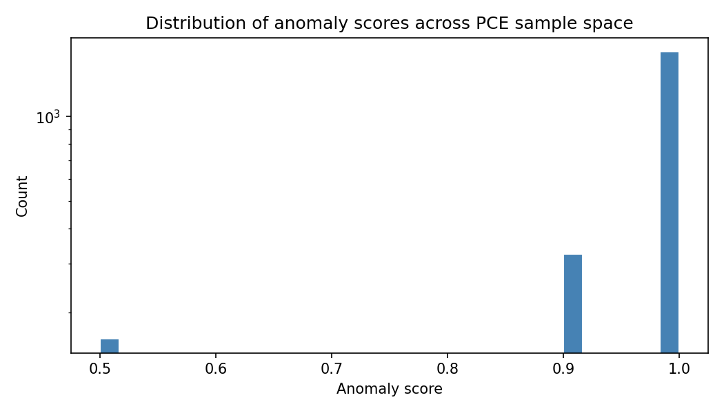
Statistical summary of the anomaly score
| Statistic | Value | What it means |
|---|---|---|
| Mean | 0.958 | The average score across all 2 187 device states sampled |
| Standard deviation | 0.097 | How much the score varies around that average |
| 10th percentile | 0.821 | 90% of sampled device states score above 0.82 |
| 90th percentile | ≈ 1.0 (capped) | The upper tail is firmly at the score cap — most devices reach the maximum |
Note: These results use calibrated input ranges (see table above) with a wider spread of error rates (0–50%) and network latency (10–1000ms), reflecting the full range of devices seen in production. The Rec-A-only run (narrower ranges, post-fix) gave mean=0.948, std=0.126; the original pre-fix run gave mean=0.91, std=0.18.
To put these numbers in plain terms: imagine sampling 2 187 real POS devices from across a fleet, spanning the full range of CPU loads, error rates, and health check outcomes that you would normally expect to see. The anomaly detector would rate:
- 9 out of 10 devices at a score of 0.82 or higher (10th percentile = 0.821)
- Most devices at or near the maximum score of 1.0
- The average device at 0.958 out of 1.0 — essentially always critical
The score distribution is heavily saturated toward 1.0. The alert fatigue problem identified in What the results mean persists and requires the weight/threshold changes in Recommendations B and C.
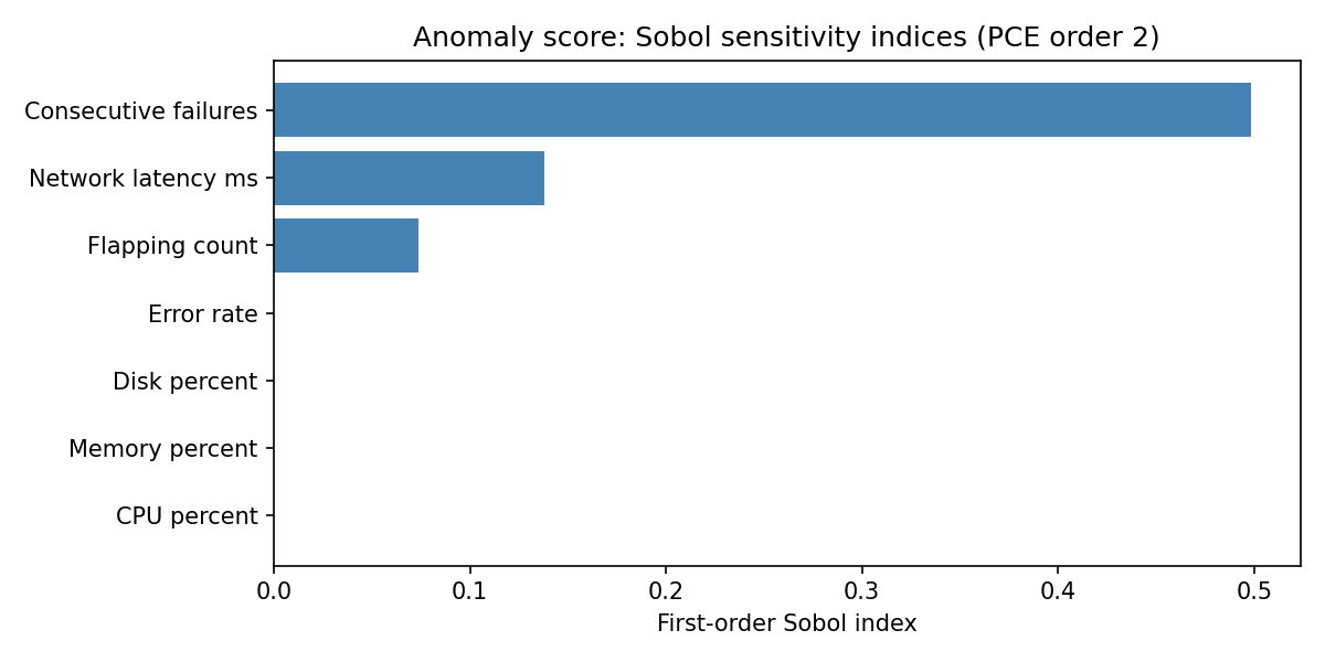
First-order Sobol sensitivity indices
Recall that a Sobol index answers: "If I vary only this metric — leaving all others fixed — what fraction of the total variability in anomaly scores does it account for?" An index of 1.0 would mean that metric alone determines all possible score variation; an index of 0.0 means the metric is completely invisible to the detector.
| Parameter | Sobol index | Share of variance | Plain-English interpretation |
|---|---|---|---|
consecutive_failures | 0.499 | ~50% | The single most decisive metric. Fires in ~80% of samples and has the highest weight (+0.80). |
network_latency_ms | 0.138 | ~14% | Second-most influential. Fires in ~81% of samples at the 200ms threshold. |
flapping_count | 0.074 | ~7% | Moderate influence. Fires in ~50% of samples. |
error_rate | 0.000 | ~0% | Effectively zero — not because error rate doesn't matter, but because it fires in ~90% of samples (see note below). |
cpu_percent | 0.000 | ~0% | Effectively invisible. Fires in only ~11% of samples; score already capped by other metrics. |
memory_percent | 0.000 | ~0% | Same as CPU. |
disk_percent | 0.000 | ~0% | Same as CPU. |
These results reflect the detector after Recommendation A was applied, run with calibrated input ranges.
Why does error_rate have a Sobol index of 0.000?
This is the key new finding from the calibrated-range run, and it is worth understanding carefully.
A Sobol index measures how much of the variance in the output is explained by varying a single parameter. Variance requires some outputs to be high and some to be low. If a metric fires in 90% of samples, it makes a near-constant contribution to the score — it is almost always adding its +0.50 weight. A near-constant input cannot contribute to variance, and therefore its Sobol index is near zero.
This is the saturation paradox:
A parameter that fires almost all the time looks statistically identical to a parameter that fires almost none of the time — both have near-zero Sobol indices. The difference is:
- A parameter that never fires doesn't affect the score at all.
- A parameter that always fires raises the baseline score for every device, inflating the mean toward 1.0 and suppressing variance.
For error_rate: with the range extended to 0–50% and a threshold of 5%, the error rate check fires in ~90% of samples. It is essentially always on, contributing a flat +0.50 to almost every score. It cannot be the "deciding factor" in any sample because it is rarely absent. Sobol = 0.
For cpu_percent, memory_percent, disk_percent: the opposite problem — thresholds set at 90% mean these checks fire in only ~11% of samples, so they rarely change the outcome in a score that is already being pushed to 1.0 by the stability metrics.
Both extremes are problems. A well-calibrated detector should have fire probabilities that are neither near 0% nor near 90% for most inputs — this is what Recommendations B and C are designed to achieve.
The first-order indices sum to ~71%. The remaining ~29% comes from interaction effects — combinations of metrics that jointly push scores to the cap.
A second finding: two silent configuration bugs (now fixed)
During analysis, the anomalously low Sobol index for network_latency_ms (0.042 despite a substantial weight of +0.40) prompted inspection of ai/anomaly_detection.py lines 38–39. The code was loading two thresholds using different dictionary keys than the ones present in ai/config.yaml:
Key in config.yaml | Key the code was looking for | Effect |
|---|---|---|
network_latency_ms: 200 | "max_latency_ms" — not found | Fell back to hardcoded 500ms |
error_rate: 0.05 | "max_error_rate" — not found | Fell back to hardcoded 0.05 |
Recommendation A has been implemented — both keys are now corrected. The latency threshold is now read correctly from config.yaml as 200ms (down from the erroneous 500ms default). The effect is clearly visible in the updated Sobol indices: network_latency_ms rises from 0.042 to 0.138, confirming that the config file is now wired to the running system.
What the results mean for the HOMEPOT system
1. One metric dominates the detector
consecutive_failures alone explains 50% of all score variance. The three hardware resource metrics combined explain only ~0% of variance in the current calibrated run (see the saturation paradox above — CPU/disk/memory fire in only ~11% of samples, so the score is already being pushed to 1.0 before they get a chance to be the deciding factor). The resource checks are nearly invisible to the scoring system at the current 90% thresholds across the calibrated input space.
- A POS device running at 95% CPU, 92% memory, 88% disk simultaneously scores 0.60 (three × 0.20). This is below a typical "critical" alert threshold.
- A device that has failed three health checks in a row scores 0.80 immediately, regardless of its resource usage.
- A device at 95% CPU with no other issues scores only 0.20 — effectively invisible to the alerting system.
This may or may not match operational intent. Consecutive health check failures are a strong signal of device unavailability. But extremely high CPU or memory usage for extended periods is also operationally significant. The current weights make availability the only thing that matters.
2. The 90% resource thresholds are effectively dead zones
At 90% CPU/memory/disk thresholds, these checks fire in only ~11% of samples. In most realistic device states, they never fire. Lowering the thresholds (or raising the weights) would make them contribute meaningfully.
3. Alert fatigue is baked in by design
With a mean score of 0.958 across all calibrated inputs, operators will receive critical alerts for 9 out of 10 device states in the input space covered by this study. This will make the alerting system unreliable in practice — if everything is critical, nothing is.
4. Config/code misalignment was detectable only by UQ
The config key bugs found during this study would not be caught by unit tests that mock the config reading, or by integration tests that only check a small number of hand-picked input combinations. The bug was only visible because the UQ analysis showed a lower-than-expected Sobol index for network_latency_ms, which prompted a detailed code inspection.
Recommended changes
Recommendation A — Fix the config key bugs (Implemented)
The two mismatched config keys in ai/anomaly_detection.py have been corrected:
"max_latency_ms"→"network_latency_ms"(matchesconfig.yamlkey)"max_error_rate"→"error_rate"(matchesconfig.yamlkey)
This ensures that changes to ai/config.yaml are actually reflected in the running system.
Recommendation B — Lower resource-metric thresholds
Lower the CPU, memory, and disk thresholds from 90% to a more operationally meaningful level (e.g. 80%) so that resource pressure fires in a larger fraction of realistic device states and contributes to score variance. This can be done solely via ai/config.yaml without touching the scoring code.
Recommendation C — Rebalance the weights
The +0.80 weight for consecutive_failures is approximately 4× the resource weights. Consider whether this extreme dominance reflects operational intent. A more balanced weighting (e.g. +0.50 / +0.30 / +0.20 tiers) would give each category a fairer share of score variance.
Recommendation D — Re-run after production telemetry is available
Replace the Uniform input distributions with distributions fitted to observed fleet telemetry. This will give production-accurate Sobol indices and may reveal additional imbalances in the current weight structure.